Efficient Access to Google Buildings V3: A Two-Step Workflow for Targeted Downloads and Processing

on July 23, 2025

Efficient access to Google buildings v3: A two-step workflow for targeted downloads and processing

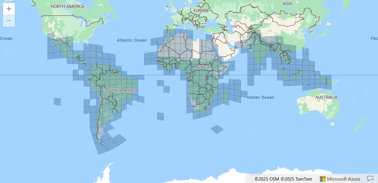
The Google Open Buildings v3 dataset is a valuable global resource containing building footprint information for the majority of the countries across the Global South, including Africa, South and Southeast Asia, and Latin America. While powerful in scope, the full dataset weighs in at 178GB in compressed form, a size that makes it impractical for many localised research or planning tasks.

Most users don’t need all of it; they need data for specific cities, countries, or project areas. Yet the official dataset is distributed in large spatial tiles, and there’s no straightforward way to download just the relevant parts.

(Google Earth Engine is a good option if your study area is a single city or two. If your study area increases in size, it is not really an option.)

In this blogpost, we present a simple, scalable, and memory-efficient two-step pipeline for working with the Google Buildings v3 dataset:

Step 1 – Tile selection and download: Identify and download only the tiles that intersect with your region of interest (ROI), using spatial filtering.
Step 2 – Tile processing and Filtering: Extract just the building footprints within your ROI, while avoiding unnecessary processing or storage of the rest.

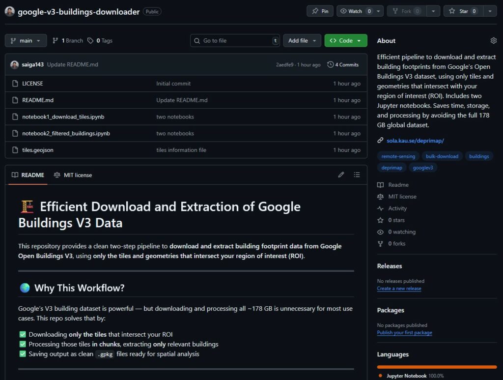
This approach works with any polygon-based ROI – whether it’s a single boundary or a set of disjoint polygons. It’s implemented in Python using open-source tools and is available through a public Github Repository.

Whether you’re working on deprivation mapping, urban morphology, or infrastructure planning, this pipeline offers a lightweight and reusable method to access only the data you actually need, and nothing more.

Github Repository link: https://github.com/saiga143/google-v3-buildings-downloader

Step 1: Discover and Download Only Relevant Tiles

The first part of this workflow is about being selective: don’t download everything -just the tiles you actually need.

Each tile in the Google v3 dataset corresponds to a 0.1° × 0.1° area and is published as a ‘.geojson.gz’ file. Google provides a public metadata file (tiles.geojson) that includes the metadata and download URL for every tile.

What this step does

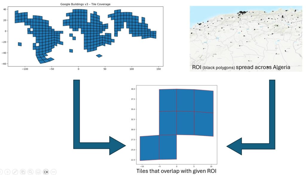
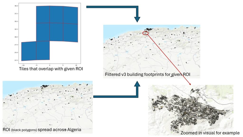
Loads your region of interest (ROI), which can be a single polygon or many disjoint polygons (see below example where I have urban clusters across Algeria).
Loads the official Google tile index.
Filters the tiles that intersect your ROI.
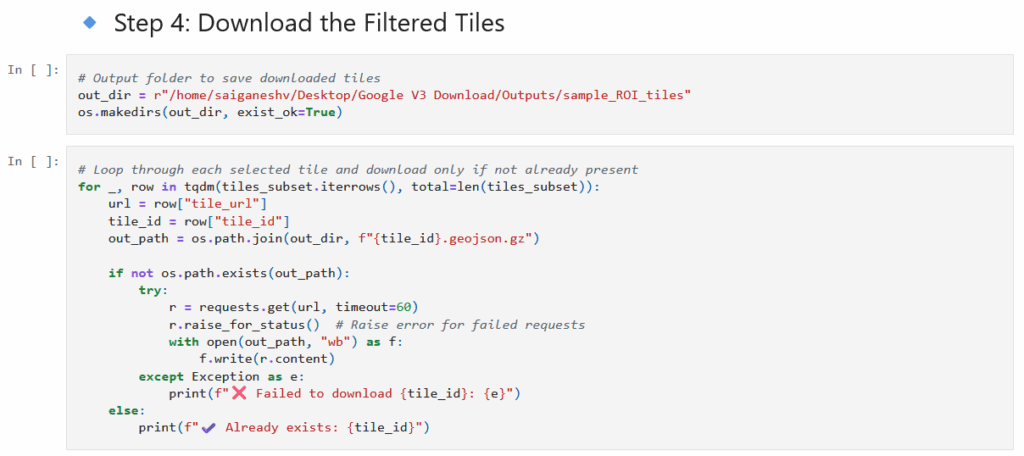
Downloads only those tiles (each saved as ‘.geojson.gz’) to a local folder.

This is fast, scalable, and avoids wasting time and storage on irrelevant data.

What you need

Your ROI file.
Google’s tiles.geojson (available in the repo)
‘notebook1_download_tiles.ipynb’ notebook in the repo

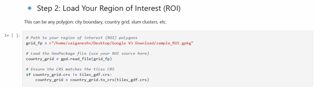
At step 2, replace the path with your ROI file path.

At step 4, replace the path for where you want to save the downloaded tiles.

Step 2: Process and Extract Buildings within your ROI

Once you’ve downloaded only the tiles that intersect your ROI, the next step is to extract just the buildings that fall within your boundary. This is important because:

Even selected tiles can cover a much larger area than your ROI
Each tile can still contain tens of thousands of building footprints
Processing or saving the entire tile results in necessary RAM use and file bloat

This step ensures that you retain only what you need.

What this step does

Reads each downloaded tile in chunks (to avoid RAM overload)
Converts geometry from WKT (Well-Known Text) format into spatial objects
Filters buildings by spatial intersections with your ROI
Writes only the filtered results into a single ‘.gpkg’ file

⚠️ Important Format Note

Although the downloaded files have a ‘.geojson.gz’ extension, they are not standard GeoJSON files. Each tile is actually a CSV file containing:

One row per building
A ‘geometry’ column with a WKT-formatted polygon
Attributes like ‘confidence’, ‘area_in_meters’, and geographic coordinates.

This means you need to:

Read the file with ‘pandas.read_csv(…)’
Parse the geometry column using ‘wkt.loads(…)’
Wrap the result into a ‘GeoDataFrame’

This nuance is not documented by Google (or at least we couldn’t find it), and most users are unaware of it. The notebook handles this automatically.

What you need

Your downloaded tiles from step 1
‘notebook2_filtered_buildings.ipynb’ notebook from the report

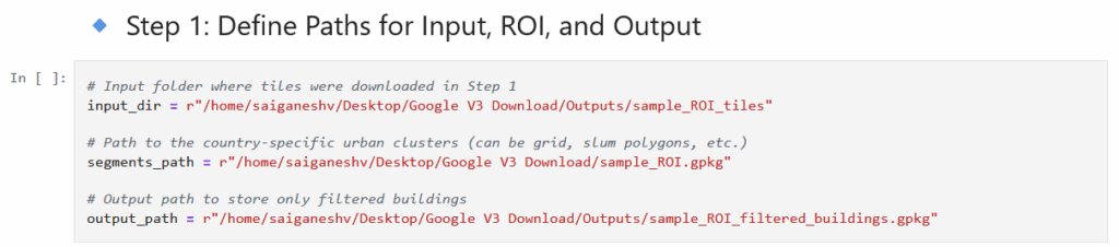
At Step 1, define the paths for your ROI, downloaded tiles for your ROI from the previous notebook and the output directory where you would like to save your final filtered buildings geopackage file for your ROI.

🌍Why this workflow matters

This two-step workflow was built out of necessity; working with the full Google Buildings v3 dataset is impractical for most real-world projects. By limiting downloads to only relevant tiles and filtering buildings strictly to your region of interest, you:

Avoid downloading or storing hundreds of unnecessary gigabytes.
Reduce memory load and processing time in every step.
Enable scalable, replicable workflows for multiple countries or cities.
Keep your outputs clean, efficient, and immediately usable.

Whether you’re working on slum detection, urban morphology, or infrastructure planning, this approach lets you focus on what matters – the data that actually intersects your study area.

Closing Thoughts

Google Open Buildings v3 is an incredibly valuable dataset – but to truly make use of it, we need tools that support selective, efficient, and scalable access. This two-step workflow makes that possible.

You can:

Clone or fork the Github repository
Use the notebooks as-is, or plug in your own region of interest
Extend the logic to batch-process multiple countries, add filters, or integrate with ML workflows.

🔗 GitHub Repository

https://github.com/saiga143/google-v3-buildings-downloader